
Results and exports#
Where are my outputs? Inside the project, in runs/<name>/. One
directory per run, named after the run. Nothing is hidden in a database,
nothing is packed into an archive: the arrays are Zarr, the tables are
Parquet, the frozen configuration is TOML, the seal and the provenance are
JSON.
The DuckDB file in .hmp/ is an index over those directories. It makes
listing, filtering and ranking fast. It is not the source of truth: delete
it and hmp catalog reindex rebuilds it from the run directories.
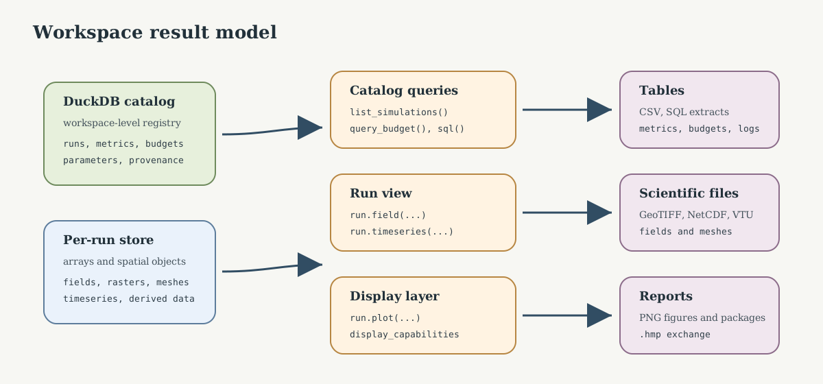
Fig. 90 The run directory holds everything a reader needs. The index answers
“which runs exist”; hmp catalog reindex rebuilds it from the seals.#
What one run writes#
<project>/
├── project.toml                  shared settings, and the marker of the project root
├── run_demo.toml                 the config you launched
├── hydromodpy.lock               frozen input data
├── runs/
│   └── nancon_intermittence_mf6/
│       ├── config.toml           frozen resolved configuration of this run
│       ├── fields.zarr/          array store: head, mesh, forcings, derived
│       ├── tables.parquet/       one Parquet file per tabular payload
│       ├── figures/              figures rendered for this run
│       ├── manifest.json         seal, written last
│       ├── provenance.json       versions, git commit, solver binary
│       ├── annotations.json      tags and notes, written after the seal
│       └── trash.json            present only while the run sits in the trash
├── sessions/
│   └── 20260726-104019-optuna-5ecea3e0/
│       ├── session.json          identity, search space, best trial
│       └── trials.jsonl          one JSON line per evaluated trial
├── share/                        on-demand exports, reports, .hmp packages
└── .hmp/                         internals: index.duckdb, logs, checkpoints, scratch
Two rules follow from that layout:
A run directory without a manifest did not finish.
manifest.jsonis written last, after every artefact it declares.A run keeps its name.
runs/<name>/is the human name of the run, with its.vNsuffix when the name was reused (aber_transient_mf6.v2).hmp catalog renamemoves the directory, then updates the index.
Reading each artefact#
tables.parquet/ with pandas#
Plain Parquet files. No HydroModPy import needed.
import pandas as pd

tables = "runs/nancon_intermittence_mf6/tables.parquet"
metrics = pd.read_parquet(f"{tables}/metrics.parquet")
budgets = pd.read_parquet(f"{tables}/budgets.parquet")
series = pd.read_parquet(f"{tables}/timeseries.parquet")
File |
Columns |
|---|---|
|
One row: the run snapshot the index rebuild reads back. |
|
|
|
Parameter name, zone, value, unit, parameterization. |
|
|
|
|
|
|
|
One row per input artefact used by the run. |
|
GeoParquet features: watershed, contour, buffered box, hydrographic networks. |
fields.zarr/ with xarray#
The array store keeps head, time and crs at the root, and groups
the rest: mesh, geographic, forcing, derived, state,
particles, meta.
Read it through hydromodpy.read(), which resolves the variable name
against the field registry and hands back a lazy xarray.DataArray:
Passing time as an int returns the eager numpy array of that
single step; leaving it out loads every persisted step lazily. sel and
bbox narrow the read further.
The store carries no dimension_names metadata, so xarray.open_zarr
on the directory raises. For raw access, open the group with zarr:
import zarr

store = zarr.open_group("runs/nancon_intermittence_mf6/fields.zarr", mode="r")
print(store.tree())
Derived fields are rebuilt at read time#
The store persists primary variables. Four fields are not stored: they are recomputed on every read, from the head and the mesh topography.
Field |
Rebuilt from |
|---|---|
|
head at the uppermost saturated layer. |
|
|
|
the surface-excess budget field when the solver writes one, otherwise the geometric criterion on the water table. |
|
the per-cell drain budget field, summed over layers, sign-corrected to a positive outflow. Needs the spatial budget to be persisted. |
They read exactly like a stored field:
water_table = hmp.read(run, "watertable_elevation", time=-1)
Because they are computed, they load eagerly and ignore laziness. That is
also why a run with no persisted budget still exposes
watertable_elevation, watertable_depth and seepage_mask, but not
outflow_drain.
manifest.json, provenance.json, annotations.json#
Three small JSON files, readable with json.load.
manifest.json:manifest_version,sealed_at,run(id, name, version, status, project),geometry(cells, layers, mesh topology, mesh hash, CRS, bbox),period,config(file and hash),artifacts[](every declared file with its role, format and size),parameters,metrics.provenance.json:tool,git(commit, dirty flag),python,platform,packages,environment(frozen package list),solver(name, version, binary path, binary SHA-256),timing.annotations.json:tagsandnotes. Written after the seal, so tagging a run never invalidates its manifest.
config.toml#
The resolved configuration of that run, after the base_config chain,
the overlays and the --set overrides. It is what hmp catalog rerun
replays and what hmp run --resume reads back.
Reading from the command line#
hmp catalog ls                        # every run of the project
hmp catalog ls --status completed --solver modflow6
hmp catalog show <ref>                # metadata, metrics, parameters
hmp catalog show <ref> --detail       # plus the Zarr store layout
hmp catalog diff <ref_a> <ref_b>      # only the keys that differ
hmp catalog query "SELECT name, solver, status FROM v_simulation_summary"
hmp report compare <ref_a> <ref_b>    # side-by-side metric table
hmp viz show <ref> <figure>           # render into runs/<name>/figures/
A reference is a run name, a versioned name (aber_transient_mf6.v2), a
unique id prefix, the full id, or a selector such as @last or
@best:nse. Inspection commands open the index read-only.
hmp catalog query runs SQL against the index. simulations stores
foreign keys (solver_id, status_id); v_simulation_summary
resolves them into readable columns, so query the view unless you need the
raw table.
Reading from Python#
import hydromodpy as hmp

catalog = hmp.open("~/ws/projects/my_basin")
run = catalog.latest()

run.name, run.solver, run.status
run.summary()                # identity, cells, layers, timesteps, duration
run.parameters               # DataFrame indexed by parameter name
run.metrics                  # DataFrame: station_id, metric_name, value
run.mass_balance             # DataFrame
run.budget()                 # DataFrame
run.timeseries("discharge")  # pandas Series indexed by time
Resolve a reference, then index the catalog:
sim_id = catalog.resolve("ab12")
run = catalog[sim_id]
List and filter:
frame = catalog.list_simulations(status="completed")
runs = catalog.find(solver="modflow6")
Cross-run SQL:
ranking = catalog.sql(
    """
    SELECT name, solver, status, duration_s
      FROM v_simulation_summary
     ORDER BY created_at DESC
    """
)
Time series and geographic features go through the same
hydromodpy.read() door:
Exporting#
hydromodpy.export() (and its run.export equivalent) picks the
format from the destination suffix, or from an explicit fmt.
hmp.export(run, "head", "share/head.nc")
hmp.export(run, "watertable_elevation", "share/wt.tif", time="last")
hmp.export(run, "head", "share/head.vtu", time="last")
hmp.export(run, "discharge", "share/discharge.csv")
Format |
Suffix |
Notes |
|---|---|---|
CSV |
|
Time series and tables. |
NetCDF |
|
Gridded fields, every timestep unless |
GeoTIFF |
|
Cloud-optimised raster. Requires a CRS on the run; pass
|
Shapefile |
|
One polygon per cell, for legacy GIS tooling. |
GeoPackage |
|
Same geometry, single-file container. |
VTU |
|
Mesh plus field, for ParaView. |
|
|
Portable package: config, provenance, fields, tables, manifest. |
The same surface from the command line:
hmp data export <project> --list
hmp data export <project> --sim <ref> --var head --netcdf --output share/head
hmp data export <project> --sim <ref> --var watertable_elevation --geotiff --resolution 50
hmp data export <project> --raster watershed_dem --geotiff
hmp data export writes into a directory (--output, default
share/<name>/), one file per variable and per timestep. --geotiff
requires --resolution here, unlike the Python call which derives the
pixel size from the grid.
Packaging a run for exchange#
hmp catalog export <ref> -o share/paper_run.hmp
hmp catalog import share/paper_run.hmp
catalog.export_package(run.sim_id, "share/paper_run.hmp")
catalog.import_package("share/paper_run.hmp")
The archive carries the frozen config, the provenance, the fields and the
tables, with checksums verified on import. The run identity survives the
round-trip, so re-importing into the same project is refused unless
--force is given.
Rebuilding the index#
hmp catalog reindex
The rebuild walks runs/ and sessions/, reads each manifest.json
and each session.json, and repopulates the index. It reports what it
found:
indexed 3 run(s) and 1 session(s)
  baseline_run
  optuna_iter_0013
  optuna_iter_0016
  20260726-104019-optuna-5ecea3e0
  calibration_iterations: 20 row(s)
  calibration_sessions: 1 row(s)
  ...
Use it after moving a project, after restoring a backup, or whenever the
index and the disk disagree. Deleting .hmp/index.duckdb loses nothing
that a rebuild cannot restore.
Temporal conventions in comparison CSV exports#
Comparison CSV files distinguish state snapshots from period values
explicitly. Read the time_role column before interpreting
time_index or elapsed_seconds.
|
Meaning |
|---|---|
|
Explicit state before the first transient period. Useful for initial-condition diagnostics, but it is not a budget period. |
|
Instantaneous model state at the reported elapsed time, for example a hydraulic-head or water-table map. |
|
Value associated with a completed period. Budget tables also provide
|
|
Row obtained by reducing several time rows, for example with a mean, min, max or sum reducer. |
For budgets, elapsed_seconds is the period end time. Do not compare a
period_value row to an initial_state row. Boussinesq histories may
store an explicit initial state at t = 0; comparison budget exports skip
that row instead of treating it as a zero-duration budget.
Comparison metrics enforce the same distinction: fallback matching can align
equivalent elapsed times or equivalent non-initial order positions, but it
must not compare rows with different time_role values. For explicit
state selection, prefer time = "initial_state" when the initial
condition itself is the target, and time = "first_computed" when the
first transient result is the target. The legacy time = "first" selector
means “first available row” and is therefore ambiguous when one solver
exports an initial state and another starts at the first computed step.
Where to look next#
Workspace layout for the workspace, project and run hierarchy and the path-resolution rules.
CLI reference for every command and its flags.
Storage Layout for the storage contract itself.
API Reference for the low-level classes and methods.